Normal distribution: normalcdf, invNorm and normalpdf in Scientific calculator plus 991 for Android
Press SHIFT 3 (DISTR) and choose normalcdf for the probability that a normal value falls between two bounds: normalcdf(lowerbound, upperbound, mean, sigma). Leave the mean and sigma out for the standard normal. invNorm runs it backwards, from an area to the value of x, and normalpdf gives the height of the bell curve. Switch to numeric calculation first, with S⇌D, or the answer comes back as an exact expression instead of a decimal.
- Menu
- SHIFT 3 (DISTR)
- Probability
- normalcdf(lowerbound, upperbound[, mean, sigma])
- Inverse
- invNorm(area[, mean, sigma])
- Defaults
- mean 0, sigma 1: the standard normal
The normal distribution has three functions on the calculator, one for each of three questions about the bell curve: how likely is a value between two bounds (normalcdf), which value has a given share of the curve to its left (invNorm), and how high is the curve at a point (normalpdf). They need no data entered in STAT mode: you give them the mean and the standard deviation directly.
The distribution menu
Press SHIFT 3 DISTR. The menu holds sixteen functions covering the normal, Student-t, chi-square, F, binomial, Poisson and geometric distributions. Type part of a name in the search box at the top of the menu to narrow the list, then choose one. Its whole name goes into the calculation; you type its arguments, and = gives the answer like any other calculation.
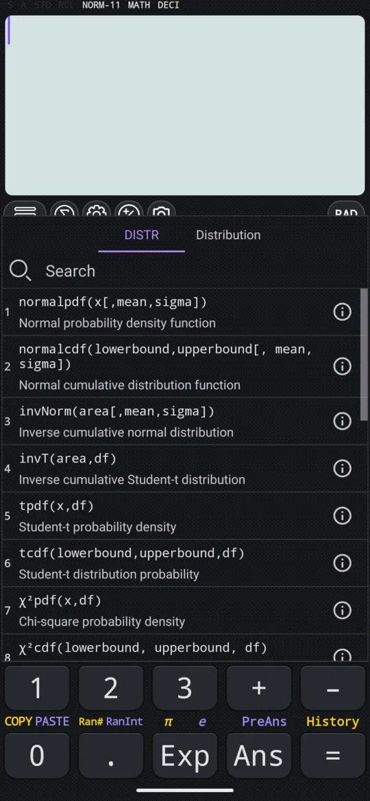
The names can also be typed letter by letter on the calculation screen, without opening the menu. The menu is quicker, since it inserts the whole name in one tap.
Every entry shows the arguments it takes, in order. Arguments inside [ ] are optional: leave them out and a standard value is used. For the normal functions, mean and sigma are the mean and the standard deviation of the distribution; left out, they are 0 and 1, which is the standard normal.
normalcdf: the probability between two bounds
normalcdf(lowerbound, upperbound[, mean, sigma]) gives the probability that a normally distributed value falls between the two bounds.
How to work out a normal probability
-
If DECI is not on the status line, press S⇌D to switch to numeric calculation.
-
Press SHIFT 3 DISTR and choose normalcdf.
-
Type the lower bound, the upper bound, the mean and the standard deviation, pressing SHIFT ) , between one and the next. Leave the last two out for the standard normal.
-
Press =.
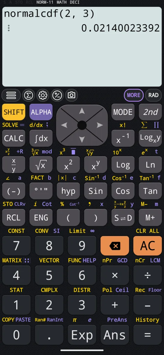
The probability that a standard normal value falls between 2 and 3:
in normalcdf(2, 3)
out 0.02140023392
The same interval on a distribution with mean 0.2 and standard deviation 0.6:
in normalcdf(2, 3, 0.2, 0.6)
out 0.0013483674
Below a value: the one-sided trick
A probability below a value needs a lower bound all the same. Put a number far below the mean where −∞ would go, such as −10⁹⁹, as the manual does. The probability that a value from a distribution with mean 35 and standard deviation 2 falls below 36:
in normalcdf(-10⁹⁹, 36, 35, 2)
out 0.69146246127
invNorm: the value behind an area
invNorm(area[, mean, sigma]) runs normalcdf backwards: given an area between 0 and 1, it returns the value of x with that area to its left. Feeding the answer above back in, shortened, returns the 36 it came from:
in invNorm(0.6914625, 35, 2)
out 36.00000021999
The standard normal value with 97.5% of the area to its left leaves 2.5% in each tail, so it is the number behind a 95% confidence interval:
in invNorm(0.975)
out 1.9599639845
normalpdf: the height of the curve
normalpdf(x[, mean, sigma]) gives the probability density at x: the height of the bell curve at that point, not a probability. For a probability over an interval, use normalcdf.
in normalpdf(3, 0.9, 2.1)
out 0.11522415453
With the mean and sigma left out, normalpdf(0) is the peak of the standard normal curve:
in normalpdf(0)
out 0.3989422804
normalcdf is the area under this curve between two bounds, the kind of area a definite integral finds under a curve you write yourself.
normalcdf or P, Q and R
STAT mode has its own normal areas: P(t), Q(t) and R(t) on the Distribution tab of the STAT menu, SHIFT 1 STAT. They work on the standard normal only, and are the natural next step after →t turns a value from your data into a standard score; Z-scores, P, Q and R covers them. normalcdf needs no data, and takes any mean and standard deviation.
At a glance
| What to use | Gives |
|---|---|
| SHIFT 3 DISTR | The distribution menu |
| normalcdf(lowerbound, upperbound[, mean, sigma]) | The probability of falling between the bounds |
| invNorm(area[, mean, sigma]) | The value with that area to its left |
| normalpdf(x[, mean, sigma]) | The height of the curve at x |
| −10⁹⁹ as the lower bound | A probability below a value |
| S⇌D | Numeric calculation, for a decimal answer |
Questions
How do I work out a normal probability?
Switch to numeric calculation with S⇌D first. Then press SHIFT 3 (DISTR), choose normalcdf, and give it the lower bound, the upper bound, the mean and the standard deviation, separated by commas: normalcdf(2,3,0.2,0.6) is 0.0013483674. Leave the last two out for the standard normal: normalcdf(2,3) is 0.02140023392.
How do I find a probability below a value?
Put a lower bound far below the mean where −∞ would go, such as −10⁹⁹, as the manual does. The probability that a value from a normal distribution with mean 35 and standard deviation 2 is below 36 is normalcdf(−10⁹⁹, 36, 35, 2), which is 0.69146246127.
How do I find the value for a given probability?
Use invNorm(area, mean, sigma), where area is the area to the left of the value you want. invNorm(0.975) is 1.9599639845, the number behind a 95% confidence interval. Feeding normalcdf's answer back in, shortened to 0.6914625, invNorm(0.6914625, 35, 2) returns 36.00000021999, the 36 it came from.
Why does my answer have Erfc in it?
Because the calculator is in symbolic calculation, which keeps answers exact, and the exact form of a normal probability is written with Erfc, the complementary error function (InverseErfc for invNorm). Press S⇌D to switch to numeric calculation and the same calculation returns a decimal.
Related pages
- Z-scores from your data the standard score of a data value, and the areas P, Q and R
- Student-t, chi-square and F distributions tcdf, invT and tpdf; χ²cdf and χ²pdf; Fcdf and Fpdf
- Binomial, Poisson and geometric probabilities binompdf and binomcdf, Poisson, geometric, lists and the whole table
- Statistics and probability which tool for which job, and what each page of the chapter covers
Written from the calculator's own manual and from the app itself, version 7.6.0; every figure is one the manual shows or a capture of the app proves. Last revised on 29 September 2026.
Bug reports and feature requests go to kimcuc@samatica.com — a person reads it.