Z-scores from your data: →t and the P, Q and R functions in Scientific calculator plus 991 for Android
The Distribution tab of the STAT menu has four functions. →t converts a value from the data in the editor into its standard score, the z-score: the value minus the mean, divided by the population standard deviation σx. P(t), Q(t) and R(t) then give an area under the standard normal curve: to the left of t, between 0 and t, and to the right of t. P(1.5) is 0.93319279873.
- Standard score
- value, then →t: (x − x̄) ÷ σx
- Left tail
- P(t), the area left of t
- From the middle
- Q(t), the area between 0 and t
- Right tail
- R(t), the area right of t: 1 − P(t)
A standard score says where a value sits in its data, counted in standard deviations from the mean: 0 at the mean, 1 one standard deviation above it, −1 one below. On the calculator, →t works it out from the data in the editor, and P, Q and R turn it into a probability read off the standard normal curve.
The Distribution tab
In STAT mode, press SHIFT 1 STAT and go to the Distribution tab. It holds four functions: P(t), Q(t) and R(t), which take a value t and return an area, and →t, which makes that t from a data value.
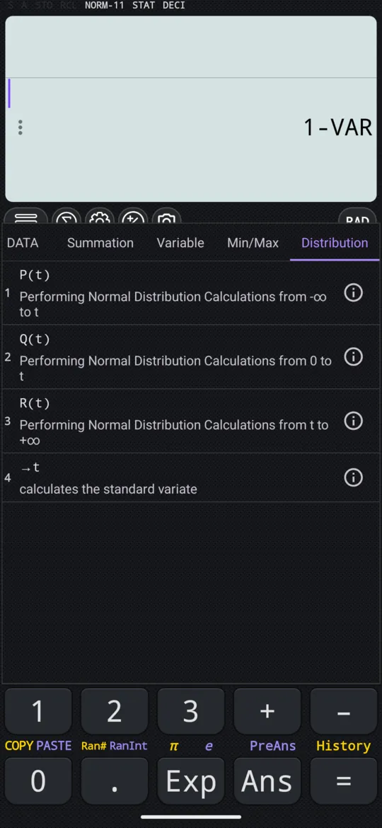
→t: the standard score of a data value
→t is postfix: the value comes first, as in 2→t. It converts a value x into its standard score by subtracting the mean of the entered x values and dividing by their population standard deviation, σx. So a value one standard deviation above the mean becomes 1, one below becomes −1, and the mean itself becomes 0, whatever the original units were.
The manual's example uses the nine values 1, 2, 2, 3, 3, 3, 4, 4 and 5, entered in 1-VAR with a Frequency column as on the statistics editor. The answers here are decimals, with numeric calculation on (DECI on the status line; see decimals for probabilities):
| x | Frequency |
|---|---|
| 1 | 1 |
| 2 | 2 |
| 3 | 3 |
| 4 | 2 |
| 5 | 1 |
How to find the standard score of a data value
-
With the data in the editor, press AC to go to the calculation screen, and type the value: 2.
-
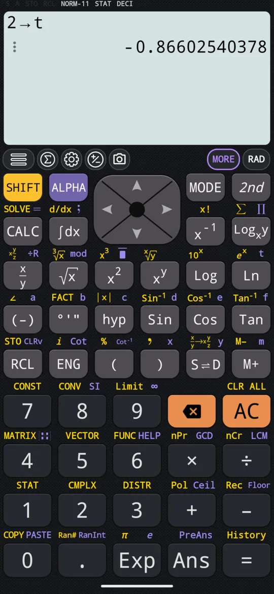
Press SHIFT 1 STAT, choose →t on the Distribution tab, then press =.
in 2→t
out -0.86602540378
The mean of this data is 3 and σx is 1.15470053838, as the 1-VAR screen shows, so 2 sits a little under one standard deviation below the mean.
Then turn that score into a probability: press SHIFT 1 STAT again, choose P(t) on the Distribution tab, which types P( on the input line, then press Ans ) =:
in P(Ans)
out 0.19323811539
That is the share of a normal curve with this mean and standard deviation that lies below 2: an estimate from the model, not a count of the nine values themselves.
P(t): the area to the left
P(t) is the area to the left of t, everything from −∞ up to it: the probability that a value falls below t.
At t = 1.5 the shaded part is almost all of the curve:
in P(1.5)
out 0.93319279873
P(0) is exactly 0.5, since half the curve lies either side of the mean.
Q(t): the area from the middle
Q(t) is the area between the mean and t, from 0 out to it: the probability that a value falls between the centre of the curve and t.
The same t = 1.5, measured from the middle instead. It is exactly P(1.5) − 0.5:
in Q(1.5)
out 0.43319279873
Q measures from the middle outward on whichever side t lies, and the curve is symmetric, so a negative t gives the same answer as its positive twin: Q(−1.5) is 0.43319279873 as well. Q(0) is 0, there being no width to measure.
R(t): the area to the right
R(t) is the area to the right of t, from t out to +∞: the probability that a value falls above t. It is what is left of the curve after P, so R(t) = 1 − P(t).
in R(1.5)
out 0.06680720127
The curve is symmetric, so R(−t) equals P(t): R(−1.5) is 0.93319279873.
Which to use
| You want | Use |
|---|---|
| The standard score of a data value | The value, then →t |
| The chance of falling below t | P(t) |
| The chance of falling above t | R(t) |
| The chance of falling between the mean and t | Q(t) |
| A normal curve with another mean and standard deviation | normalcdf, on SHIFT 3 DISTR |
At a glance
| Keys | What they give |
|---|---|
| SHIFT 1 STAT, Distribution, P(t) | The area left of t |
| SHIFT 1 STAT, Distribution, Q(t) | The area between 0 and t |
| SHIFT 1 STAT, Distribution, R(t) | The area right of t |
| A value, then SHIFT 1 STAT, Distribution, →t | Its standard score in the entered data |
Questions
How do I find a z-score on the calculator?
Enter the data in STAT mode, press AC to leave the editor, type the value, then choose →t on the Distribution tab of the STAT menu (SHIFT 1) and press =. →t comes after the value, as in 2→t. It subtracts the mean of the data and divides by its population standard deviation σx, so a value one standard deviation above the mean gives 1.
What is the difference between P, Q and R?
All three measure an area under the standard normal curve, each over a different part of it. P(t) is the area to the left of t, from −∞ up to it; Q(t) is the area between the mean (0) and t; R(t) is the area to the right, from t to +∞, so R(t) = 1 − P(t). At t = 1.5, P is 0.93319279873, Q is 0.43319279873 and R is 0.06680720127.
Do P, Q and R use the mean and standard deviation of my data?
No. They use the standard normal curve, mean 0 and standard deviation 1, however the editor is filled; your data comes in only through →t, which turns a data value into a standard score first. For a normal curve with another mean and standard deviation, use normalcdf on SHIFT 3 (DISTR), not the Distribution tab.
How do I find the probability below a z-score?
Use P(t) on the Distribution tab: P(1.5) is 0.93319279873, the probability that a standard normal value falls below 1.5. Straight after →t, P(Ans) gives the probability below the data value you just standardised.
Related pages
- Mean, standard deviation, variance and quartiles from your data x̄, σx and sx, variance, n, quartiles and the median
- Normal distribution normalcdf, invNorm and normalpdf, and the one-sided trick
- Entering data in STAT mode the editor, the Frequency column, inserting and deleting rows
- Statistics and probability which tool for which job, and what each page of the chapter covers
Written from the calculator's own manual and from the app itself, version 7.6.0; every figure is one the manual shows or a capture of the app proves. Last revised on 29 September 2026.
Bug reports and feature requests go to kimcuc@samatica.com — a person reads it.