Statistics and distributions in Scientific calculator plus 991 for Android
Numbers go into a table - one column for single-variable work, two for paired data, and a frequency column beside them for repeats. From there the STAT mode returns means, standard deviations and a five-number summary, or fits one of seven regression models and draws the curve through the points. A separate distribution menu holds sixteen functions covering the normal, Student-t, chi-square, F, binomial, Poisson and geometric distributions, each with its density and its cumulative probability, and an inverse for the normal and the t.
§ i The statistics editor
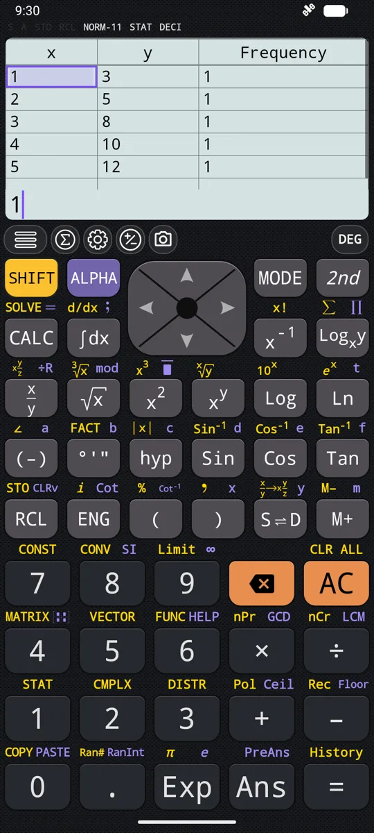
The editor is a table and nothing more. One column for 1-VAR, two columns, x and y, for a paired type, and a Frequency column after them holding the number of times each row is repeated. Nothing is written to a cell until the equals key is pressed; equals then moves down one row in the same column and appends a fresh row when the one just filled was the last, so a column is entered straight down without touching the arrow keys.
- A cell accepts an expression as well as a number: entering 2+3 stores 5
- Committing a row with cells still blank fills them in - a blank x or y becomes 0, a blank Frequency becomes 1
- DEL removes the row the selection sits on; SHIFT AC removes every row; the Edit tab also inserts a row, which has no key of its own
- Arrowing onto a cell shows its value and the next key typed replaces it; tapping the cell edits what is already there instead
- The frequency column can be turned off under Settings → Calculation → STAT/DISTR, though turning it off discards the frequencies already entered
- Entered data outlives the mode: it survives leaving STAT and it is saved when the app closes
- A row with a cell still blank is dropped before the calculation runs, so the trailing blank row left by the last equals does no harm
in A+B·ln(X) fitted to (170, 66), (173, 68), (179, 75)
out a = −852.16277461319, b = 178.68979688248, r = 0.99198632129
r close to 1 says the curve follows the three points closely.
§ ii Single-variable data and seven regression models
One menu governs the whole mode. Under DATA ► Type of statistical calculation sit eight types: single-variable, and seven regression models. The one in use carries a tick, and choosing a type opens the editor for it. Single-variable and paired-variable data are kept apart, so switching between the two loses neither, and switching among the paired types keeps the same x and y columns and simply refits them.
- 1-VAR - single variable (x)
- A+BX - linear regression, y = a + bx
- A+BX+CX^2 - quadratic regression, y = a + bx + cx²
- A+B·ln(X) - logarithm regression, y = a + b·ln(x)
- Ae^(BX) - e exponential regression, y = a·e^(bx); A·B^X - ab exponential regression, y = a·b^x
- A·X^B - power regression, y = a·x^b; A+B/X - inverse regression, y = a + b/x
- The STAT menu opens with SHIFT 1 (STAT) and reopens on whichever tab was used last. It works only in the STAT/DISTR mode, chosen with MODE; anywhere else the same key reports Supported only in STAT mode
§ iii Mean, standard deviation and the five-number summary
DATA ► 1-variable calculation or DATA ► 2-variable calculation puts every statistic on screen at once, to eleven decimal places. Which of the two is offered follows the calculation type. Single-variable data gives thirteen values - the mean, the two sums, the population and sample spreads, the count, and the five-number summary. Paired data gives twenty-three: the quartiles are dropped, and the y column, the cross sums and the higher powers of x take their place.
To find the mean and standard deviation of a column of numbers
- 1. Press MODE and select STAT/DISTR.
- 2. Press SHIFT 1 (STAT) and choose DATA ► Type of statistical calculation ► 1-VAR. The editor opens on an x column.
- 3. Type each value and press =; the selection drops to the next row. A value that repeats can go in once, with its count in the Frequency column.
- 4. Press SHIFT 1 (STAT) again and choose DATA ► 1-variable calculation. x̄ is the mean, σx the population standard deviation and sx the sample standard deviation.
- Single-variable: x̄, ∑x, ∑x², σ²x, σx, s²x, sx, n, min(x), Q1, Med, Q3, max(x). The last five are the five-number summary, Med being the median
- Paired adds ȳ, ∑y, ∑y², σ²y, σy, s²y, sy, ∑xy, ∑x³, ∑x²y, ∑x⁴, min(y), max(y)
- σ is the population form and s the sample form, so σ²x divides by n and s²x by n − 1. For the x column of the example below - 170, 173 and 179 - that gives σ²x = 14 and s²x = 21, σx = 3.74165738677 and sx = 4.58257569496
- A value that cannot be worked out is printed as Indeterminate rather than raising an error - a single row does this to s²x and sx, since dividing by n − 1 divides by zero
- Regression results come from DATA ► Regression calculation: a and b, the correlation coefficient r, and RegEQ, the whole fitted equation with its numbers filled in
- The quadratic type is the exception: it adds c and reports R², the coefficient of determination, in place of r
in 2-variable calculation on (170, 66), (173, 68), (179, 75)
out x̄ = 174, ∑x = 522, ∑x² = 90870, σ²x = 14, σx = 3.74165738677, s²x = 21, sx = 4.58257569496, n = 3, ȳ = 69.66666666667, ∑y = 209, ∑y² = 14605, σ²y = 14.88888888889, σy = 3.85861230093, s²y = 22.33333333333, sy = 4.72581562625, ∑xy = 36409, ∑x³ = 15826056, ∑x²y = 6345647, ∑x⁴ = 2757580722, min(x) = 170, max(x) = 179, min(y) = 66, max(y) = 75
Twenty-three values from three rows of data, each to eleven decimal places.
§ iv Every statistic is also a variable
A statistic does not have to be read off a summary screen. Choosing one from the STAT menu drops its symbol into the calculation being typed, and equals evaluates it, so x̄ or sx or ∑xy can stand on its own or sit inside a longer expression. The variables are grouped across the tabs of the menu, and the ones marked paired appear only when a paired-variable type is selected.
- Summation: ∑x, ∑x², ∑x³, ∑x⁴, and for paired data ∑y, ∑y², ∑xy, ∑x²y
- Variable: x̄, σ²x, σx, s²x, sx, n, and for paired data ȳ, σ²y, σy, s²y, sy
- Min/Max: min(x), Q1, Med, Q3, max(x), and for paired data min(y) and max(y)
- Regression, paired only: a, b, r, x̂, ŷ, RegEQ - the quadratic type adds c, reports R² in place of r, and offers x̂1 and x̂2 in place of x̂
- n is the total of the frequency column rather than the number of rows, so it is not always a whole number
- Q1, Med and Q3 describe single-variable data; they stay on the Min/Max tab while a paired type is selected, but the value they return there is not a quartile, so switch to 1-VAR before reading them
- r measures the model that was chosen, not the raw columns: fitting A+B·ln(X) to (20, 3150), (110, 7310), (200, 8800) and (290, 9310) gives r = 0.99833446826, the correlation of ln(x) with y, while the correlation of x with y is only 0.92284790164
in x̄ with x = {1, 2, 3, 4, 5} and Frequency = {1, 2, 3, 2, 1}
out 3
The frequency column counts each row without repeating it.
§ v Estimating y from x, and the regression graph
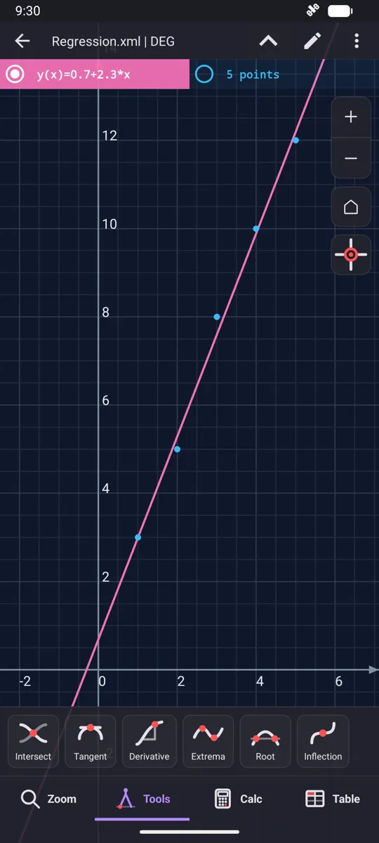
Once a paired regression has been fitted, the model can be read in either direction. ŷ turns a value of x into the y the model predicts, and x̂ turns a value of y back into the x that produces it. Both are postfix operators - the value comes first and the operator after it, so the estimate of y at x = 160 is typed 160 ŷ rather than ŷ(160). DATA ► Regression graph then draws the entered points and the fitted curve through them. Here the curve is drawn for you; to plot a function of your own, or build a table of values from it, see graphing and tables.
- ŷ estimates y from a given x; x̂ estimates x from a given y
- Quadratic regression offers x̂1 and x̂2 in place of x̂, because a parabola reaches most heights twice
- The estimate is read from whichever regression is currently in force, so the model has to be fitted first
- The regression graph plots every entered pair and overlays the fitted function, for any of the seven paired models
- For the quadratic fit to (1, 3), (2, 4), (6, 12), (7, 16), (12, 47), (33, 300), the curve drawn is y = 1.2914492945845226 + 0.5346717681561088x + 0.2582285157785109x²
in 160 ŷ
out 8106.89798497268
The model was y = −3857.9844132709 + 2357.53155139817·ln(x), and ln(160) is about 5.0751738, which is where the estimate comes from.
§ vi The z-score of a data value: →t, P, Q and R
Four functions sit on the Distribution tab of the STAT menu. Three of them - P, Q and R - take a value t and return an area under the standard normal curve, differing only in which part of the curve they measure. The fourth, →t, converts a value from the entered data into that t - its standard score, or z-score - by subtracting the mean of the x column and dividing by its population standard deviation σx. P, Q and R always work on the standard curve, mean 0 and standard deviation 1, whatever is in the editor; the entered data reaches them only through →t.
- P(t) is the area to the left of t, everything from −∞ up to it: P(1.5) = 0.93319279873, and P(0) is exactly 0.5
- Q(t) is the area between the mean and t: Q(1.5) = 0.43319279873, which is P(1.5) − 0.5
- Q is always positive, so Q(−1.5) is 0.43319279873 as well, and Q(0) is 0
- R(t) is the area to the right of t, and R(t) = 1 − P(t): R(1.5) = 0.06680720127
- The curve is symmetric, so R(−t) equals P(t) - R(−1.5) is 0.93319279873
- →t is postfix, as in 2→t: a value one standard deviation above the mean becomes 1, one below becomes −1, and the mean itself becomes 0, whatever the original units were
in 2→t
out -0.86602540378
With x = {1, 2, 3, 4, 5} and Frequency = {1, 2, 3, 2, 1} in the editor, P(Ans) then returns 0.19323811539.
§ vii Normal distribution: normalpdf, normalcdf, invNorm
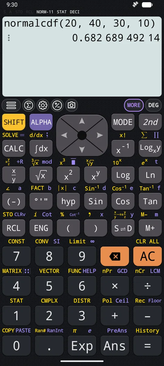
SHIFT 3 (DISTR) opens the distribution menu, and typing part of a name narrows the list. Each entry is a plain function: choosing it drops the whole name into the calculation being typed, and the answer arrives on equals like any other. The names can also be typed letter by letter without opening the menu at all. Arguments inside square brackets are optional - leave mean and sigma out and they are 0 and 1, which is the standard normal. A cumulative probability is an area under the density curve, the kind of area a definite integral finds under a curve you write yourself.
To work out a normal probability
- 1. If the calculator is in symbolic calculation (FRAC), press S⇌D to switch to numeric. Left symbolic, the answer comes back full of Erfc.
- 2. Press SHIFT 3 (DISTR), type part of the name to narrow the list, and choose normalcdf.
- 3. Enter the lower bound, the upper bound, the mean and the standard deviation, in that order and separated by commas. Leave the last two out for the standard normal.
- 4. For a probability below a value there is no −∞ to type, so use a lower bound far below the mean, such as −10⁹⁹.
- 5. Press =.
- normalpdf(x[,mean,sigma]) - the height of the bell curve at x, not a probability: normalpdf(3,0.9,2.1) = 0.11522415453, and the peak normalpdf(0) = 0.3989422804
- normalcdf(lowerbound,upperbound[, mean, sigma]) - the probability of falling between the two bounds: normalcdf(2,3) = 0.02140023392 on the standard normal, and normalcdf(2,3,0.2,0.6) = 0.0013483674
- invNorm(area[,mean,sigma]) - runs normalcdf backwards, from the area to the left of a point to the value of x that point sits at
- invNorm(0.975) = 1.9599639845, the number behind a 95% confidence interval
in normalcdf(-10^99,36,35,2)
out 0.69146246127
Feeding that area back in as invNorm(0.6914625,35,2) returns 36.00000021999, the 36 it came from.
§ viii Student-t, chi-square and F
These three take degrees of freedom instead of a mean and a standard deviation. The t functions accept any df greater than 0; chi-square wants a whole number greater than 0; and the F functions take two, a numerator and a denominator, because the F distribution compares two variances. A chi-square or F value is never negative, so a left-hand tail starts its interval at 0 rather than at a large negative bound.
- tpdf(x,df) - Student-t probability density: tpdf(2.2,2) = 0.05590051995
- tcdf(lowerbound,upperbound,df) - Student-t probability over an interval: tcdf(-2,3,18) = 0.9657465611
- invT(area,df) - runs tcdf backwards, from an area to a t-value, the number a printed t-table would give
- χ²pdf(x,df) - chi-square density: χ²pdf(2,9) = 0.01581361895
- χ²cdf(lowerbound, upperbound, df) - chi-square probability: χ²cdf(0,19.023,9) = 0.97500196014, the 97.5% point on 9 degrees of freedom
- Fpdf(x, numerator df, denominator df) - F density: Fpdf(2,24,19) = 0.13436820209, and Fpdf(5,4,3) = 0.02671503274
- Fcdf(lowerbound, upperbound, numerator df, denominator df) - F probability: Fcdf(0,2.4523,24,19) = 0.97499895769, the 97.5% point with 24 and 19 degrees of freedom
in invT(0.95,24)
out 1.71088207991
In symbolic calculation the same expression returns something full of InverseBetaRegularized, so switch to numeric with S⇌D first.
§ ix Binomial, Poisson and geometric
These three describe counts rather than measurements, so x is a whole number. A pdf gives the probability of exactly one outcome and a cdf adds up every outcome from the bottom to x. Any of them takes a list in the x slot to answer several questions at once, and the binomial pair will hand back the whole table when x is left out entirely.
- binompdf(numtrials,p[,x]) - exactly x successes in numtrials independent trials: binompdf(8,0.7,3) = 0.04667544
- binomcdf(numtrials,p[,x]) - x successes or fewer: binomcdf(5,0.6,3) = 0.66304, and binomcdf(5,0.6,{3,4,5}) = {0.66304, 0.92224, 1}
- poissonpdf(mean,x) - exactly x events where mean were expected; the mean comes first: poissonpdf(6,10) = 0.04130309341
- poissoncdf(mean,x) - x events or fewer: poissoncdf(0.126,{0,1,2,3}) = {0.88161484678, 0.99269831748, 0.99969657613, 0.999990503}
- geometpdf(p,x) - the first success arrives on trial x: geometpdf(0.4,6) = 0.031104
- geometcdf(p,x) - the first success arrives on trial x or earlier: geometcdf(0.5,{1,2,3}) = {0.5, 0.75, 0.875}
- In symbolic calculation these stay exact - 2072/3125, 486/15625, {1/2, 3/4, 7/8}, or 2916/(175e⁶) for the Poisson - so press S⇌D for a decimal
in binompdf(5,0.6)
out {0.01024,0.0768,0.2304,0.3456,0.2592,0.07776}
Reading along it: 0 successes has probability 0.01024, one has 0.0768, and so on up to all five at 0.07776.
Questions
How do I work out a normal distribution probability?
Use normalcdf from the distribution menu, SHIFT 3 (DISTR), giving it the lower bound, the upper bound, the mean and the standard deviation: normalcdf(2,3,0.2,0.6) is 0.0013483674. Leave the last two out for the standard normal. For a probability below a value, use a lower bound such as −10⁹⁹, and switch to numeric calculation with S⇌D first, or the answer comes back full of Erfc. invNorm runs it backwards: invNorm(0.975) is 1.9599639845.
How do I find the mean and standard deviation of a set of numbers?
In STAT/DISTR mode, choose the 1-VAR type, enter the numbers down the editor's x column, then choose DATA ► 1-variable calculation from the STAT menu, SHIFT 1 (STAT). x̄ is the mean, σx the population standard deviation and sx the sample standard deviation. A value that repeats need only be entered once, with its count in the Frequency column.
How do I find an inverse t value without a printed table?
Use invT(area, df) from the distribution menu: it runs the t distribution backwards and returns the t-value a printed table would give. invT(0.95, 24) is 1.71088207991. Switch to numeric calculation with S⇌D first - in symbolic calculation the same expression is kept exact and comes back full of InverseBetaRegularized rather than as a number.
Which regression models can it fit?
Seven, alongside single-variable work: linear, quadratic, logarithm, e exponential, ab exponential, power and inverse. A fit returns a and b, the correlation coefficient r, and RegEQ, the whole equation with its numbers filled in; the quadratic type is the exception, adding c and reporting R² in place of r. DATA ► Regression graph then plots the entered points with the fitted curve through them.
How do I work out a chi-square probability?
Choose χ²cdf from the distribution menu, SHIFT 3 (DISTR), and give it a lower bound, an upper bound and the degrees of freedom: χ²cdf(0, 19.023, 9) is 0.97500196014, the 97.5% point on nine degrees of freedom. The name carries the χ² character, so the menu is the practical way to enter it. A chi-square value is never negative, so a left-hand tail starts at 0, and the degrees of freedom must be a whole number greater than 0.
Can it return the whole binomial table at once?
Yes. Leave the count out and binompdf(5,0.6) returns every outcome in order: {0.01024, 0.0768, 0.2304, 0.3456, 0.2592, 0.07776}, from none of the five up to all of them. A list in the x slot works too, for the Poisson and geometric functions as well - binomcdf(5,0.6,{3,4,5}) gives {0.66304, 0.92224, 1}.
Why does my standard deviation show Indeterminate?
Because the sample forms divide by n − 1, and with a single row of data that is a division by zero. s²x and sx are printed as Indeterminate rather than raising an error, while the population forms σ²x and σx, which divide by n, still have values. Enter a second row and all four appear.
Does the entered data stay after leaving the statistics mode?
It does - the table survives leaving STAT and is saved when the app closes. One limitation is worth knowing: the frequency column can be turned off under Settings → Calculation → STAT/DISTR, and turning it off discards the frequencies already entered. Switching it back on returns blank cells, not the old numbers.
Elsewhere in the manual
- i. Calculus integrals, derivatives, limits, series
- ii. Graphing and tables curves, shaded areas, tables of values
- iii. Equations and inequalities polynomials, systems, intervals
- iv. Matrices and vectors determinants, eigenvalues, products
- v. Everything else the calculator does the whole index
Written from the calculator’s own manual for version 7.6.0, and every worked example is one that manual shows. Last revised on 25 September 2026.
Bug reports and feature requests go to kimcuc@samatica.com — a person reads it.