Graphing and tables in Scientific calculator plus 991 for Android
Every graph starts the same way: type the expression on the input line, then press GRAPH. What comes back depends on what you typed - a wave, a five-petal rose, a tilted ellipse, a shaded arch - and TABLE mode turns the same kind of function into a column of values instead. The picture is not decoration; a limit that reads Indeterminate on the calculation screen becomes obvious the moment you watch the two sides of the curve run off in opposite directions.
§ i Plot a function, or several on one graph
There is no separate graphing mode to enter and no y= list to fill in first: the expression goes on the ordinary input line, right-hand side only, and GRAPH draws it. Several functions go on one pair of axes if a semicolon separates them, and each is drawn as its own curve. To keep drawing fast the grapher reads a reduced syntax rather than the calculator's full one.
To plot a function
- 1. If the function is trigonometric, set the angle unit to Radian first with the RAD key at the top of the display; in Degree, Sin(x) is drawn as Sin(πx/180), which is not the curve asked for.
- 2. Type the right-hand side only, with no y and no equals sign; x is ALPHA then the ) key.
- 3. For a second curve, press ALPHA then the ∫dx key for a semicolon, and type the next function.
- 4. Press GRAPH.
- Sin(x) draws y = sin x; the y and the equals sign are left off
- Arithmetic: plus, minus, multiply, divide, power and factorial
- Six trigonometric functions and six hyperbolic ones, each paired with its inverse
- Square root, cube root, e^x, Ln(x) to base e and Log(x) to base 10
- Floor(x), Ceil(x) and |x| for rounding and absolute value
- Two constants, π and e
- The graph always calculates in radian, whatever the angle unit is set to
in Sin(x);Cos(x)
out Both curves drawn together on one pair of axes, each in its own colour
The same semicolon later separates the x and y halves of a parametric pair, so it is worth learning where it sits.
§ ii Cartesian and polar coordinates
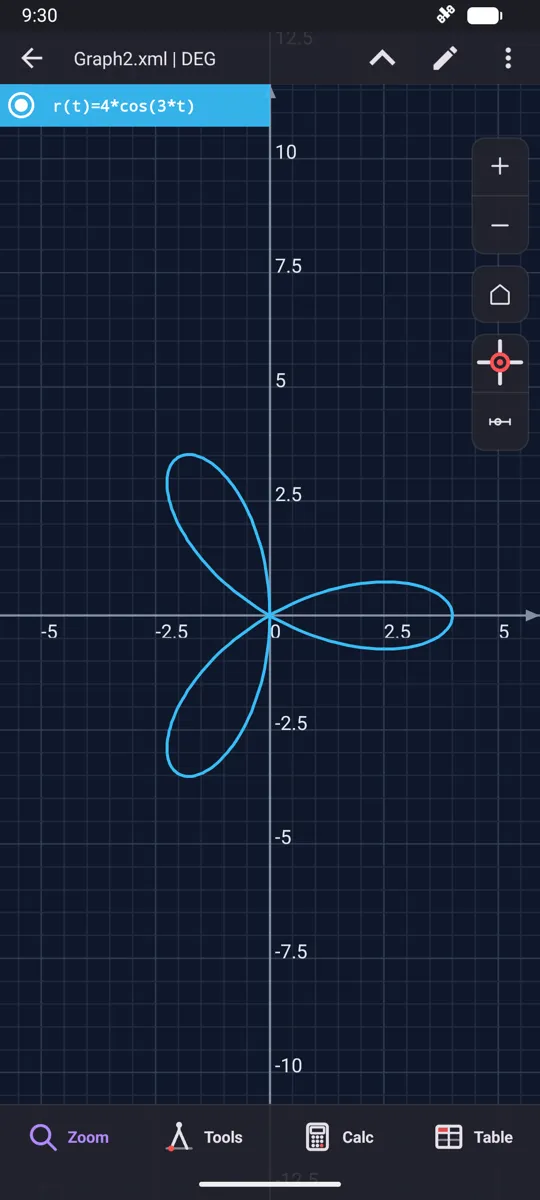
The coordinate system is a setting rather than a different tool. In Cartesian the expression gives y for each x; in Polar it gives a radius for each angle, and you type t wherever you would write theta. The grid tells you which one you are in - Cartesian rules the plane into squares, Polar into circles about the origin.
- Change the coordinate system in the graph settings
- Cartesian: the expression is y as a function of x
- Polar: the expression is r, the radius, as a function of t, the angle measured from the x-axis
- 2Sin(5x) in Cartesian is a wave
- The same formula written in t closes into a five-petal rose in Polar
in 2Sin(5t)
out A five-petal rose about the origin
The formula is the same but for its letter - what changed is which quantity the plane is measuring.
§ iii Parametric curves in t
A parametric graph is a Cartesian graph whose x and y are each a function of a parameter t. Give the two functions with x first and a semicolon between them. Because neither coordinate is tied to the other, the curve is free to double back on itself in a way no single y(x) could manage.
- x(t);y(t) - the x function, the semicolon, then the y function
- t is the same parameter the polar grapher uses
- The curve need not pass the vertical-line test
- t^2;t^3 draws x = t squared and y = t cubed
in t^2;t^3
out The curve with x = t², y = t³
Squaring y and cubing x both give t⁶, so every point on this curve satisfies y² = x³.
§ iv Implicit curves and shaded inequalities
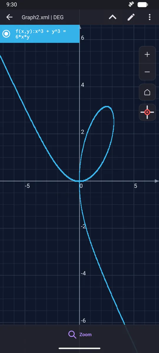
Type a whole equation, with x and y anywhere on either side. Nothing has to be solved for y first, so an ellipse - which is not a function of x at all - draws as readily as a line. Replace the equals sign with a comparison and you get a shaded region instead of a curve, and the semicolon puts the two on one plot.
- f(x,y) = g(x,y), with x and y in any arrangement on either side
- x^2+y^2-x*y=4 draws a tilted ellipse
- x+2y>3 shades the half-plane rather than drawing only its boundary
- Five comparisons are available: greater than, greater than or equal to, equal to, less than, less than or equal to
- The comparison operators work only in implicit graphs
- Implicit graphs take the semicolon separator too, so an equation and an inequality can share one plot
in x^2+y^2-x*y=4;x+2y>3
out The tilted ellipse with the shaded half-plane laid across it
Read the overlap directly: the points that satisfy both are the arc of the ellipse lying inside the shading.
§ v Shade the area under a curve
An integral can be drawn instead of evaluated. The template is filled in exactly as it would be for a number, and GRAPH takes the place of equals: the curve is plotted, the region between the two limits is shaded, and both limits are marked on the x-axis. The shaded region is the answer, which is also the quickest way to explain a sign that looks wrong - area below the x-axis counts as negative, so an integral across a hump and a dip returns the difference between them rather than the total ink on the page.
To shade the area under a curve
- 1. Press ∫dx and choose Integral; the template arrives with four empty slots.
- 2. Type the expression in the first slot.
- 3. Move between the slots with the left and right arrow keys, or tap one; the variable slot already holds x.
- 4. Fill in the lower limit and the upper limit.
- 5. Press GRAPH rather than equals.
- Four slots, the same as for a number: expression, variable, lower limit, upper limit
- The whole curve is plotted; only the region between the limits is shaded
- Both limits are marked as points on the x-axis
- Area below the axis is subtracted from the area above it, not added to it
- Equals on the same template gives the value itself; definite integrals as exact numbers are on the calculus page
in ∫dx ► Integral: Sin(x), x, 0, π, then GRAPH
out Sin(x) plotted, the arch from 0 to π shaded, both limits marked on the x-axis
Press equals on the same template instead and the answer, in Radian, is 2 - the area of the shaded arch.
§ vi A curve and its derivative on one graph
Either entry in the derivative menu can be drawn instead of evaluated: fill in the template as for an answer, then press GRAPH. Derivative at a point draws four things at once - the expression solid, its derivative dashed and in a colour of its own, and a labelled point on each at the chosen value. Reading the two curves together is the point of the drawing. Wherever the dashed curve crosses zero the solid one has a peak or a trough, and where the dashed curve is high the solid one is climbing steeply.
- SHIFT then ∫dx opens the derivative menu; GRAPH takes the place of equals
- The point on f'(x) is the answer the calculation screen gives; the point on f(x) shows where on the curve that slope was measured
- Each marked point takes the colour of the curve it sits on
- Derivative, the entry with no point, draws the same pair of curves with nothing marked: for 1/x, the curve solid and −1/x² dashed
- Where the dashed curve is positive the solid one rises; where it is negative the solid one falls
- For the slope as a number, and how the angle unit changes it, see derivatives at a point
in SHIFT ∫dx ► Derivative at a point: x^3+x^2, x, 2, then GRAPH
out f(2)=12 on the solid curve, f'(2)=16 on the dashed one
The dashed curve is 3x²+2x, the derivative written out; f'(2)=16 is the slope, and f(2)=12 marks where on the curve it was taken.
§ vii Graph a limit and read it from both sides
A limit is drawn the same way: fill in the Lim template and press GRAPH instead of equals. The curve is plotted and a dashed vertical line marks the point x is heading towards; follow the curve to the line from each side and read off the height it aims for. The picture earns its keep where the curve breaks, because a limit that does not exist is just as plain to see as one that does.
- SHIFT then 9 opens the limit menu; Lim(expr, x→a) has three slots - expression, variable, point
- GRAPH plots the curve with a dashed vertical line at the point
- sin(x)/x has no value at 0, yet both sides climb towards 1, which is the answer equals gives
- 1/(x−1) at 1 runs off in opposite directions, so there is no single height to head for
- The graph shows at a glance what an answer of Indeterminate means
- One-sided limits and limits at infinity give the numbers behind the picture
in SHIFT 9 ► Lim(expr, x→a): 1/(x−1), x, 1, then GRAPH
out 1/(x−1) plotted with a dashed line at x = 1; the two sides run off in opposite directions
Press equals on the same template and the answer is Indeterminate - the drawing is what the word means.
§ viii Solver graphs: roots, turning points and solution bands
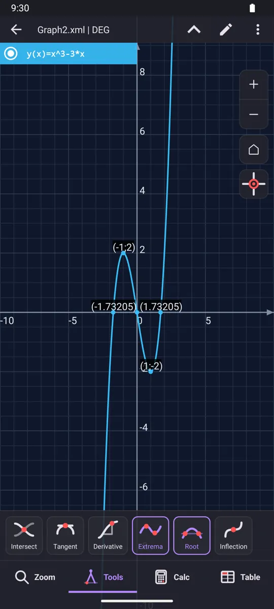
Press GRAPH in the polynomial solvers at any time - while entering coefficients or while reading a solved result - and the polynomial in the editor is plotted with its roots and turning points already marked, and from degree 3 up its inflection points too. Each marker can be switched on or off from the graph screen's own controls. The inequality solvers mark the roots and add a shaded vertical band running the full height of the plot, whose left and right edges sit at the roots - that band, and not the area between the curve and the axis, is the solution set.
- Equations of degree 2 to 5, plotted from whatever coefficients are currently in the editor
- Degree 2 marks the roots and the vertex; degrees 3, 4 and 5 add the inflection points
- x³ − 6x² + 11x − 6 opens with its roots, turning points and inflection point marked
- x⁵ − 15x⁴ + 85x³ − 225x² + 274x − 120 gets the same treatment
- Inequalities of degree 2 to 4 draw the curve with its roots marked and the solution set shaded
- For x² − x − 2 > 0 two bands cover x < −1 and 2 < x; for the same polynomial with < 0 a single band covers −1 < x < 2
- From the statistics editor, SHIFT 1 (STAT) then Regression graph draws a regression curve through a set of data points, for paired data only
in Solve polynomial of degree 2: a = 1, b = −2, c = −3, then GRAPH
out y = x² − 2x − 3 with its roots x = −1 and x = 3 and its minimum at (1, −4) marked
The parabola opens upward because a = 1 is positive, so the turning point is a minimum rather than a maximum.
§ ix TABLE: a column of values over a range
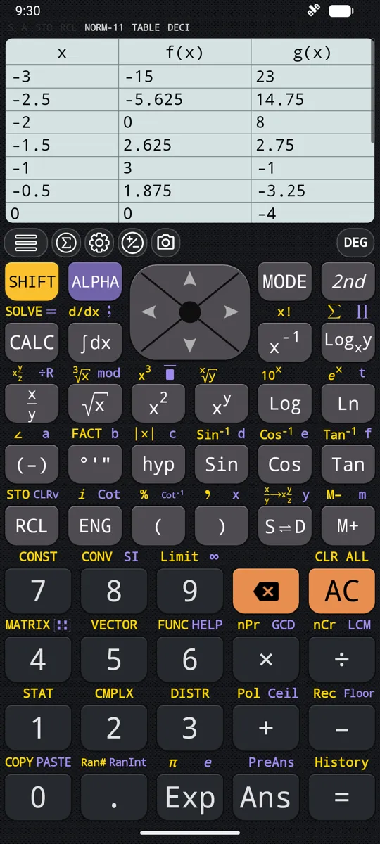
Choose TABLE from MODE. It evaluates a function at every value of x from a first value to a last, stepping by a fixed amount, and lays the results out as a table. A second function can be tabulated beside the first, so two functions can be compared row by row. The prompts arrive one at a time, each holding the value it was given last time, and NEXT and PREV walk back and forth over them without losing any.
- Five inputs - f(x), g(x), Start, End and Step - each accepted with the equals key
- Nothing is evaluated along the way; the press that accepts Step generates the whole table
- Start, End and Step accept any real expression, not only plain numbers: 1/2, π and √2 all work
- A negative step walks the range downwards, so Start 5, End 1 and Step −1 gives x = 5, 4, 3, 2, 1
- Both ends belong to the table when the step divides the distance exactly, so 1 to 5 by 1 is five rows rather than four
- S⇌D regenerates the table in FRAC or DECI - √x over 0 to 4 gives 0, 1, √2, √3, 2 rather than a column of decimals
- Tap a value in the f(x) or g(x) column to see its other formats; AC returns to the f(x)= prompt with all five inputs intact
in f(x) = x^2, g(x) = 2x, Start = 1, End = 5, Step = 1
out x: 1, 2, 3, 4, 5 | f(x): 1, 4, 9, 16, 25 | g(x): 2, 4, 6, 8, 10
The two columns cross at x = 2, where both read 4 - the kind of thing a table shows before a graph does.
Questions
How do I graph a function?
Type the right-hand side on its own - no y and no equals sign - and press GRAPH. There is no separate graphing mode to enter and no y= list to fill in first; x is ALPHA then the ) key. To put several functions on one pair of axes, type them one after another with a semicolon between them, which is ALPHA then the integral key. The grapher reads a reduced syntax: arithmetic, powers and factorial, the six trigonometric and six hyperbolic functions with their inverses, square and cube roots, e^x, Ln, Log, Floor, Ceil and absolute value.
Can it graph implicit equations like x^2 + y^2 - xy = 4?
Yes. Type the whole equation with x and y anywhere on either side; nothing has to be solved for y first, so x^2+y^2-x*y=4 draws a tilted ellipse even though it is not a function of x. Replace the equals sign with a comparison and you get a shaded region instead of a curve, so x+2y>3 shades the half-plane rather than drawing only its boundary. Five comparisons are available - greater than, greater than or equal to, equal to, less than, less than or equal to - and they work only inside implicit graphs.
How do I draw a polar graph?
Change the coordinate system to Polar in the graph settings, then type r as a function of t and press GRAPH. The expression gives r, the radius, for each t, the angle measured from the x-axis, so you type t wherever you would write theta. 2Sin(5x) in Cartesian is a wave, and the same formula written in t closes into a five-petal rose in Polar. The grid tells you which system you are in: Cartesian rules the plane into squares, Polar into circles about the origin.
How do I graph parametric equations?
Type the x function, then a semicolon, then the y function, each written in the parameter t, and press GRAPH. Typing t^2;t^3 draws the curve with x = t squared and y = t cubed. It is the same t the polar grapher uses and the same semicolon that puts two ordinary functions on one plot. Because neither coordinate is tied to the other, the curve need not pass the vertical-line test.
Does the graph use degrees or radians?
Radians, always, whatever the angle unit is set to. In Degree mode Sin(x) is translated to Sin(πx/180), so the curve drawn is not the one asked for; switch to Radian with the RAD key at the top of the display before graphing anything trigonometric. Calculations on the ordinary screen differ: a definite integral and a derivative at a point follow the angle unit, while limits, the antiderivative and the symbolic derivative always work in radian.
How do I shade the area under a curve?
Fill in the Integral template from the ∫dx menu as you would for a number, then press GRAPH instead of equals. The curve is plotted, the region between the two limits is shaded, and both limits are marked on the x-axis. Area below the x-axis counts as negative, so an integral across a hump and a dip returns the difference between them rather than the total ink on the page.
Can I graph an equation I have just solved?
Yes: press GRAPH in the polynomial solver at any time, while typing the coefficients or while a result is on screen. The polynomial is plotted from the coefficients in the editor with its roots and turning points marked, and from degree 3 up its inflection points as well. In an inequality mode the curve is drawn with its roots marked, and the solution set is shaded as a vertical band whose edges sit at the roots.
How many rows can a table of values have?
Up to 201 with the setting as it comes: the limit is 200 steps, and a table has one more row than it has steps. Rows = (End - Start) / Step + 1, because both ends belong to the table when the step divides the distance exactly. The limit is the Maximum number of entries setting, under Settings → Calculation → TABLE; a value outside 50 to 300 is pulled back to the nearer end of that range.
Elsewhere in the manual
- i. Calculus integrals, derivatives, limits, series
- ii. Equations and inequalities polynomials, systems, intervals
- iii. Statistics and distributions regression, normal, t, binomial
- iv. Matrices and vectors determinants, eigenvalues, products
- v. Everything else the calculator does the whole index
Written from the calculator’s own manual for version 7.6.0, and every worked example is one that manual shows. Last revised on 25 September 2026.
Bug reports and feature requests go to kimcuc@samatica.com — a person reads it.