Matrices and vectors in Scientific calculator plus 991 for Android
The calculator keeps two ways of doing linear algebra. MATRIX and VECTOR Mode each hold four named variables, so a matrix entered once is afterwards used by name rather than retyped; the second keyboard page types the same operations straight into an ordinary calculation, for an answer you need once and will not need again. Both give exact results wherever exact results exist - 2/3 rather than 0.667, and a length left as the square root of 14.
§ i Two ways in - the modes and the second keyboard
MATRIX Mode and VECTOR Mode are the storing route. You put a matrix into a variable, give it a name, and spend the rest of the session combining names rather than retyping numbers. The second keyboard is the other route: a row of matrix keys and a linear algebra menu sitting on the ordinary calculation screen, where each matrix is typed into the expression itself and nothing is kept afterwards. Which one to use is a question of whether the matrix has a second job to do.
- MODE opens the calculation-mode dialog; MATRIX and VECTOR are two of the entries in it.
- In MATRIX Mode one menu holds everything, opened with SHIFT 4 (MATRIX): NAMES inserts a variable, EDIT opens it in the editor, MATH lists the functions. VECTOR Mode has the same menu on SHIFT 5 (VECTOR).
- On the second keyboard there are no MatA to MatD variables - each matrix is typed directly into the calculation.
- Seven keys on the second page carry the matrix template, Det, Rank, Inverse, EiValues, the dot operator and the linear algebra menu; the digits, + - × ÷, AC and = all stay on the first page.
- Press 2nd to turn the page and 1st to turn back; the second page has its own SHIFT, ALPHA and cursor keys, so you can move around a matrix without turning back.
- The linear algebra menu is a searchable list of about sixty functions, filtered from a box at the top.
- The dot key between two matrices is the matrix product - the same answer the × key gives.
in [[1,2],[3,4]] • [[2,1],[1,2]]
out [[4,5],[10,11]]
Order matters: the same two matrices the other way round are usually a different answer. Matrices are written here row by row; on screen each one is a grid from the template key.
§ ii Storing a matrix: MatA to MatD
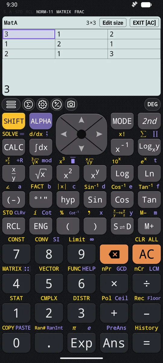
MATRIX Mode works with matrices of up to seven rows by seven columns, stored in MatA, MatB, MatC and MatD. A fifth variable, MatAns, holds the last matrix result, so an answer can be carried into the next calculation without being typed again. The editor is a grid of cells; = confirms one and moves to the next, left to right and row by row.
To store a matrix and find its determinant
- 1. Press MODE and choose MATRIX.
- 2. Press SHIFT 4 (MATRIX) and choose MatA under EDIT.
- 3. Tap Edit size and pick 2×2 from the grid.
- 4. Type 2 = 1 = 1 = 1 = to fill the cells, left to right and row by row.
- 5. Tap EXIT [AC], or press AC, to return to the calculation screen; the elements are kept.
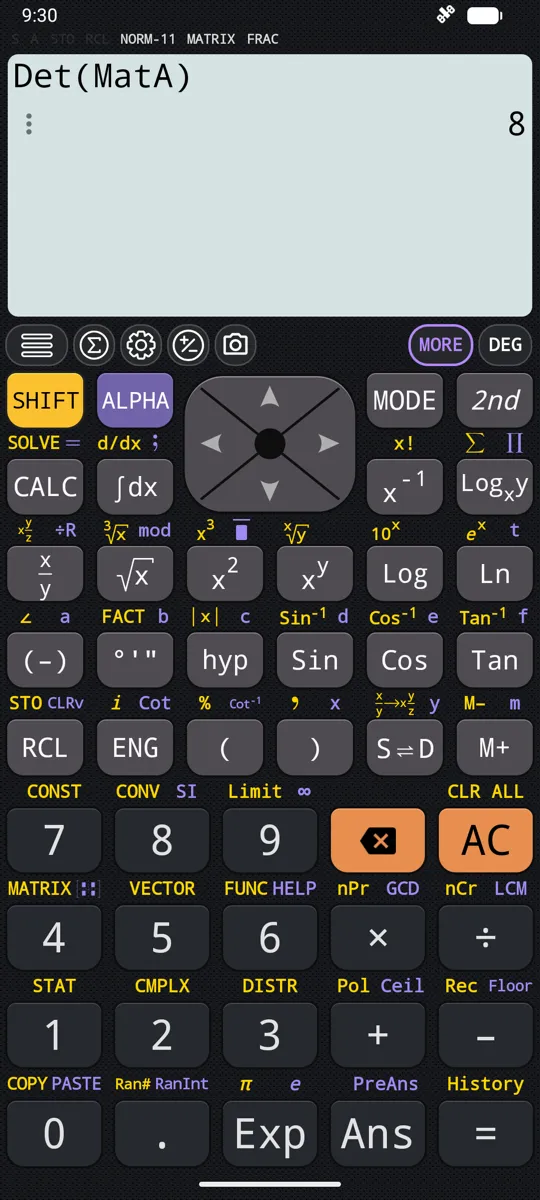
- 6. Press SHIFT 4 (MATRIX) and choose Det(matrix) under MATH, then SHIFT 4 (MATRIX) again and MatA under NAMES.
- 7. Press =. Det(MatA) comes back as 1.
- Four variables - MatA, MatB, MatC and MatD - each holding a matrix from 1×1 up to 7×7.
- Edit size opens a grid of sizes; the editor then shows one cell per element.
- An element may be a whole expression - a fraction, or the square root of 2 - and = evaluates it in place.
- Resizing a matrix later keeps the elements that still fit and puts 0 in every new cell.
- MatAns holds the last matrix result and has no pencil icon: the calculator writes it, and it cannot be edited by hand.
- SHIFT RCL (STO) and then the destination key - (-) for MatA, °'" for MatB, hyp for MatC, Sin for MatD - copies the matrix in the editor into that variable, then switches the editor to the copy.
- The NAMES list shows each variable's current size, such as [2×2], beside its name.
in MatA × MatD, where MatA = [[2,1],[1,1]] and MatD = [[1,2,3],[4,5,6]]
out [[6,9,12],[5,7,9]]
The two sizes only have to meet in the middle: columns of the first against rows of the second, and the result takes the outer two.
§ iii Determinant, inverse and transpose
Det takes a square matrix of any size and returns one number, which is also the test of whether the matrix can be inverted at all. The inverse comes either from the reciprocal key or from Inverse, and its elements are kept as exact fractions wherever that is possible. Transpose flips a matrix over its diagonal, and the size flips with it.
- Det(matrix) returns a single number and works at any square size: Det([[1,2,3],[4,5,6],[7,8,10]]) is -3.
- A determinant of 0 means the matrix has no inverse.
- The reciprocal key and Inverse(matrix) give the same answer; elements stay exact fractions where possible. On the second page, [ ]⁻¹ inserts Inverse( rather than a power.
- Transpose(matrix) turns rows into columns, so a 2×3 matrix comes back 3×2.
- The square key and the power key raise a square matrix to a power.
- IdentityMatrix(dimension) builds the square identity of the size you give - 1s down the diagonal, 0s everywhere else.
- Det, Inverse and powers all need a square matrix; the determinant of a 2×3 matrix reports an error.
in Inverse([[2,1],[1,2]])
out [[2/3,-1/3],[-1/3,2/3]]
Det of the same matrix is 3, not 0, so the inverse exists; its elements stay as exact thirds rather than rounded decimals.
§ iv Rank, trace and row reduction
Rank counts how many rows of a matrix are genuinely independent of each other, which is the question behind most "does this system have a unique solution" exercises. Trace adds the elements down the main diagonal and, unlike the determinant, does not insist on a square matrix. Row reduction is the one that does real work on a syllabus: write the coefficients and the constants of a system as a single matrix, reduce it, and read the answers out of the last column. If only the values are wanted, the equation solver takes the same rows as a grid of coefficients, for two to four unknowns, and reports each value in turn.
- The Rank key inserts MatrixRank(, which counts the independent rows; a matrix whose second row is twice its first has rank 1.
- SHIFT Rank (Trace) inserts Tr(, the sum of the main diagonal, and it works on rectangular matrices too.
- Diagonal(matrix), from the linear algebra menu, lists the elements that Tr adds up.
- SHIFT [ ]⁻¹ (RowReduce) reduces a matrix to its simplest row form.
- LinearSolve(matrix, right) solves a system directly, and LeastSquares(matrix, right) gives the best fit for an over-determined one; to fit a line or curve to paired data, use regression and curve fitting in STAT mode instead.
- NullSpace(matrix) and PseudoInverse(matrix) sit in the same menu for the cases where there is no single solution.
- In MATRIX Mode, MatrixRank and RowReduce come from the MATH section and take a stored matrix by name; the 3×3 matrix [[1,2,3],[4,5,6],[7,8,10]] has rank 3, with no redundant row.
in RowReduce([[1,2,5],[3,4,11]])
out [[1,0,1],[0,1,2]]
The rows were x + 2y = 5 and 3x + 4y = 11, so the last column reads x = 1 and y = 2.
§ v Eigenvalues and eigenvectors
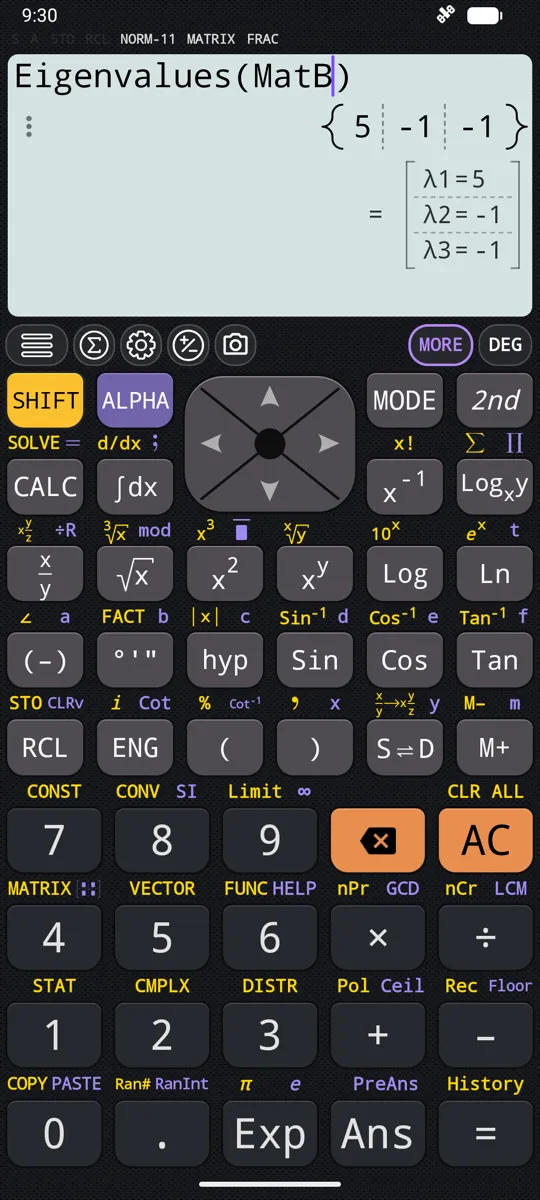
Eigenvalues and eigenvectors share one key on the second page: EiValues on its own, EiVectors with SHIFT. The answers come back in matching order, so the first row of the eigenvector result belongs to the first eigenvalue. The pieces of a diagonalisation are all here - the characteristic polynomial, the eigenvalues, the eigenvectors that form the change-of-basis matrix, and DiagonalMatrix to assemble the middle factor.
To find the eigenvalues of a matrix
- 1. Press 2nd to turn to the second page.
- 2. Press EiValues; Eigenvalues( appears on the line.
- 3. Press the matrix template key and choose 2 rows and 2 columns.
- 4. Press 1st for the digits, then type 2, right, 1, right, 1, right, 2 to fill the grid row by row.
- 5. Press right once more to leave the matrix, then press =. The eigenvalues come back as {3, 1}.
- 6. For the eigenvectors, press SHIFT EiValues (EiVectors) at step 2 instead.
- EiValues inserts Eigenvalues( and SHIFT EiValues (EiVectors) inserts Eigenvectors(.
- Each row of the Eigenvectors answer is the direction belonging to one eigenvalue, in the same order as the eigenvalues came out.
- CharacteristicPolynomial(matrix, var) gives the polynomial whose roots those eigenvalues are.
- DiagonalMatrix(list) builds a matrix from a list of diagonal elements, which is the middle factor once the eigenvalues are known.
- Both Eigenvalues and Eigenvectors need a square matrix.
- LUDecomposition, QRDecomposition and SingularValueDecomposition are in the same menu, with Adjugate, Minors, MatrixPower and MatrixExp.
- Eigenvalues and Eigenvectors are listed in MATRIX Mode’s MATH section too, alongside LUDecomposition and SingularValueDecomposition.
in Eigenvectors([[2,1],[1,2]])
out [[1,1],[-1,1]]
Eigenvalues of the same matrix are 3 and 1, so (1, 1) belongs to 3 and (-1, 1) belongs to 1.
§ vi Storing a vector: VctA to VctD
VECTOR Mode handles vectors in two and three dimensions, held in VctA, VctB, VctC and VctD, with VctAns keeping the last vector result. Choosing a variable under EDIT opens a dimension dialog first, and after that the editor is a single row of cells. On the second keyboard the same vectors are typed inline instead, with no variable behind them.
- Four variables - VctA to VctD - each 2-dimensional or 3-dimensional.
- The dimension dialog offers 1 x 2 and 1 x 3; re-opening it and picking the other size resizes the vector, keeping what fits and filling any new cell with 0.
- A component may be a full expression; = evaluates it and moves to the next cell.
- VctAns holds the last vector result and cannot be edited by hand.
- Addition and subtraction need both vectors to have the same dimension; × against a number scales the vector.
- On the second keyboard, SHIFT v2 inserts an empty 2-dimensional vector and ALPHA v3 an empty 3-dimensional one.
- Pressing the template key on its own inserts a matrix rather than a vector - a one-row matrix looks identical on screen, and the dot and cross functions reject it.
in Projection((1,2), (3,4))
out (33/25, 44/25)
The projection is the shadow of the first vector along the direction of the second, kept as fractions rather than rounded.
§ vii Dot and cross products
The dot product of two vectors is a single number, and the operator for it is the dot key, taken from the MATH section in VECTOR Mode or straight from the second page. The cross product is the × key between two vectors, or the Cross function, and the two agree. What the cross product returns depends on how many dimensions you gave it.
- Dot inserts the • operator; (1, 2) • (3, 4) is 1×3 + 2×4 = 11.
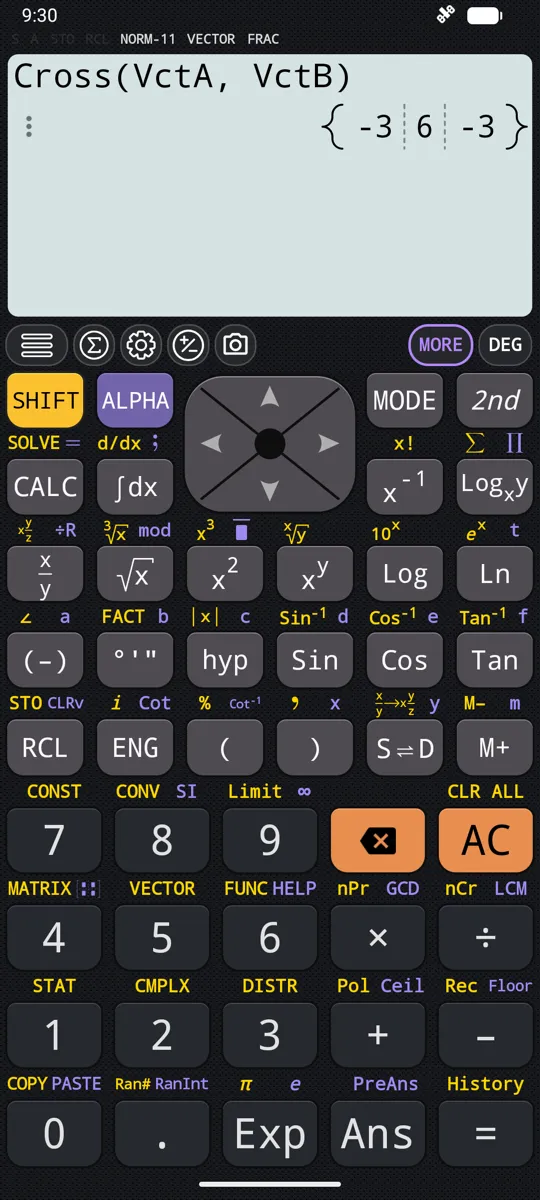
- × between two vectors is the cross product, and Cross(vector1, vector2) gives the same answer.
- Two 3-dimensional vectors give a vector perpendicular to both.
- Two 2-dimensional vectors give a single number: the vectors lie in a plane, so only the perpendicular component is left, and (1, 2) × (3, 4) is 1×4 - 2×3 = -2.
- A dot product between a 2-dimensional and a 3-dimensional vector is rejected with an error message.
- × only means the cross product while both sides are vectors entered with the template. Multiply a stored answer instead and it multiplies component by component, with no error shown.
- Use Cross(vector1, vector2) whenever either side is a stored value; it always gives the cross product.
in (2, -1, 2) × (1, 0, -1)
out (1, 4, 1)
The result is perpendicular to both inputs; the same keys on two 2-dimensional vectors would return a single number instead.
§ viii Length, angle, unit vector and distance
The measuring functions live in the linear algebra menu on the second keyboard, and in the MATH section in VECTOR Mode under slightly different names. Lengths stay exact where they can: the length of (1, 2, 3) comes back as a square root rather than a rounded decimal, and tapping the result switches to the decimal form. Angles follow whatever angle unit is currently set, so it is worth checking that before reading one.
- Norm(v) gives the length of a vector; Norm((3, 4)) is 5, and Norm((1, 2, 3)) is the square root of 14.
- VectorAngle(u, v) on the second keyboard - Angle(vectorA, vectorB) in VECTOR Mode - gives the angle between two vectors in the current angle unit.
- Two perpendicular vectors give exactly 90 in degrees, in two dimensions and three alike: (3, 4) against (-4, 3), or (1, 2, 3) against (1, 1, -1).
- Normalize(v) scales a vector to length 1 while keeping its direction; (3, 4) becomes (3/5, 4/5).
- Tapping a normalised result switches between the decimal form and the exact fractions.
- Projection(vector1, vector2) gives the shadow of the first vector along the second.
- EuclideanDistance(u, v), from the SHIFT linear algebra (clustering) menu, gives the straight-line distance between the two points the vectors reach.
in EuclideanDistance((3,4), (1,1))
out √13
That is the square root of (3-1)² + (4-1)², left as a surd rather than rounded.
§ ix Size mismatches and silent errors
Most of the trouble in matrix work is arithmetic that never happened. The calculator is quiet about it: where there is nothing to compute it shows the expression back unchanged rather than an answer, and only the genuinely impossible cases raise an error. Counting rows and columns is almost always faster than looking anywhere else.
- Addition and subtraction need matrices of exactly the same size; mix a 2×2 with a 2×3 and the expression comes back unchanged.
- Multiplication needs the columns of the first matrix to match the rows of the second.
- Det, Inverse, powers, Eigenvalues and Eigenvectors all need a square matrix; the determinant of a 2×3 matrix reports an error.
- A dot product between vectors of different dimensions is rejected with an error message.
- An unevaluated vector subtraction may reappear as an addition of the negated vector - that is still the expression, not a result.
- The dot operator and Cross reject a one-row matrix, which is why the vector templates and the plain matrix template are worth keeping apart.
- The NAMES list shows each stored size, such as [2×2], which is the quickest place to look when an answer is not the one you expected.
in {1,2,3} × {1,5,7}
out {1,10,21}
No error is shown; Cross({1,2,3},{1,5,7}) gives {-1,-4,3}, the cross product, whatever the two sides were stored as.
Questions
How large a matrix can the calculator handle?
MATRIX Mode works with matrices from 1×1 up to seven rows by seven columns, held in four variables named MatA, MatB, MatC and MatD. A fifth, MatAns, keeps the last matrix result, so an answer can go into the next calculation without being typed again. Resizing a matrix later keeps the elements that still fit and puts 0 in every new cell. The NAMES list shows each variable's current size, such as [2×2], beside its name.
How do I find the inverse of a matrix?
Press the reciprocal key, ▪⁻¹, after the matrix, or use Inverse(matrix); both give the same answer, with elements kept as exact fractions where possible. In MATRIX Mode, with MatA stored as [[2,1],[1,1]], MatA⁻¹ gives [[1,-1],[-1,2]]. On the second keyboard the [ ]⁻¹ key inserts Inverse( instead, and Inverse([[2,1],[1,2]]) gives [[2/3,-1/3],[-1/3,2/3]]. Only a square matrix with a non-zero determinant has an inverse, so if Det comes back as 0 there is none to find.
Does it work with vectors in three dimensions?
VECTOR Mode handles two-dimensional and three-dimensional vectors, and only those - the dimension dialog offers 1 x 2 and 1 x 3, with nothing above that. Four variables, VctA to VctD, hold them, and VctAns keeps the last vector result. Norm, VectorAngle, Normalize, Projection and EuclideanDistance all work at either dimension, and lengths stay exact where they can: Norm((1, 2, 3)) comes back as the square root of 14 rather than a rounded decimal. Angles are reported in whatever angle unit is currently set, so it is worth checking that before reading one.
Can it find eigenvalues and eigenvectors?
Yes. One key on the second keyboard page carries the pair - EiValues inserts Eigenvalues(, and SHIFT EiValues (EiVectors) inserts Eigenvectors( - and both need a square matrix. The answers come back in matching order, so the first row of the eigenvector result belongs to the first eigenvalue: Eigenvectors([[2,1],[1,2]]) gives [[1,1],[-1,1]] against eigenvalues 3 and 1. CharacteristicPolynomial and DiagonalMatrix sit in the same menu when the whole diagonalisation is wanted.
How do I solve a system of equations by row reduction?
Write the coefficients and the constants as one matrix and reduce it. RowReduce([[1,2,5],[3,4,11]]) returns [[1,0,1],[0,1,2]], so the rows x + 2y = 5 and 3x + 4y = 11 read out of the last column as x = 1 and y = 2. LinearSolve(matrix, right) does the same job in one step, and LeastSquares(matrix, right) gives the best fit when the system is over-determined. If you only want the values, the equation solver takes the same coefficients as a grid for two to four unknowns.
How do I get the cross product of two vectors?
The × key between two vectors entered with the vector template is the cross product, and Cross(vector1, vector2) gives the same answer. Two three-dimensional vectors return a vector perpendicular to both; two two-dimensional ones return a single number, so (1, 2) × (3, 4) is 1×4 - 2×3, or -2. There is one trap worth knowing: × means the cross product only while both sides are vectors entered with the template, and applied to stored lists it multiplies component by component with no error shown. Use Cross whenever either side is a stored value.
Why does a matrix calculation come back unchanged instead of giving an answer?
Because the sizes do not meet, and the calculator is quiet about it - where there is nothing to compute it shows the expression back rather than an answer. Addition and subtraction need matrices of exactly the same size, and multiplication needs the columns of the first to match the rows of the second. Only the genuinely impossible cases raise an error: the determinant of a 2×3 matrix, or a dot product between a two-dimensional and a three-dimensional vector. Counting rows and columns in the NAMES list is almost always faster than looking anywhere else.
Elsewhere in the manual
- i. Calculus integrals, derivatives, limits, series
- ii. Graphing and tables curves, shaded areas, tables of values
- iii. Equations and inequalities polynomials, systems, intervals
- iv. Statistics and distributions regression, normal, t, binomial
- v. Everything else the calculator does the whole index
Written from the calculator’s own manual for version 7.6.0, and every worked example is one that manual shows. Last revised on 25 September 2026.
Bug reports and feature requests go to kimcuc@samatica.com — a person reads it.